[MachineLearning] 캐글 타이타닉
머신러닝 - 캐글 타이타닉 문제 해결하기
캐글 타이타닉
위 링크는 캐글 데이터 분석 경진대회의 타이타닉호 탑승객의 생존여부를 예측하는 과제이다.
목차
데이터 불러오기
링크에서 데이터를 받아와야한다. 데이터는 이미 훈련셋과 테스트셋으로 나뉘어져 있으며 테스트 셋에는 라벨이 되는 생존여부에 대한 데이터가 없다.
데이터의 특성은 이와 같다.
| Variable | Definition | Key |
|---|---|---|
| Survival | 생존여부 | 0 = No, 1 = Yes |
| Pclass | 탑승권 등급 | 1 = 1st, 2 = 2nd, 3 = 3th |
| Sex | 성별 | male, female |
| Age | 나이 | |
| SibSp | 형제 또는 배우자 동승여부 | |
| Parch | 부모 또는 자녀 동승여부 | |
| ticket | 티켓 번호 | |
| fare | 지불 요금 | |
| Cabin | 객실 번호 | |
| Embarked | 탑승 항구 | C = Cherbourg, Q = Queenstown, S = Southampton |
데이터 분석을 위한 numpy, pandas 라이브러리를 불러온 후 https://github.com/ageron/data/raw/main/titanic.tgz 에서 파일을 받아 read_csv 메서드를 통해 가져온다.
- train_df : 훈련셋
- test_df : 테스트 셋
from pathlib import Path
import pandas as pd
import tarfile
import urllib.request

def load_titanic_data():
    tarball_path = Path("datasets/titanic.tgz")
    if not tarball_path.is_file():
        Path("datasets").mkdir(parents=True, exist_ok=True)
        url = "https://github.com/ageron/data/raw/main/titanic.tgz"
        urllib.request.urlretrieve(url, tarball_path)
        with tarfile.open(tarball_path) as titanic_tarball:
            titanic_tarball.extractall(path="datasets")
    return [pd.read_csv(Path("datasets/titanic") / filename)
            for filename in ("train.csv", "test.csv")]

train_df, test_df = load_titanic_data()
train_df.head()
| PassengerId | Survived | Pclass | Name | Sex | Age | SibSp | Parch | Ticket | Fare | Cabin | Embarked | |
|---|---|---|---|---|---|---|---|---|---|---|---|---|
| 0 | 1 | 0 | 3 | Braund, Mr. Owen Harris | male | 22.0 | 1 | 0 | A/5 21171 | 7.2500 | NaN | S |
| 1 | 2 | 1 | 1 | Cumings, Mrs. John Bradley (Florence Briggs Th... | female | 38.0 | 1 | 0 | PC 17599 | 71.2833 | C85 | C |
| 2 | 3 | 1 | 3 | Heikkinen, Miss. Laina | female | 26.0 | 0 | 0 | STON/O2. 3101282 | 7.9250 | NaN | S |
| 3 | 4 | 1 | 1 | Futrelle, Mrs. Jacques Heath (Lily May Peel) | female | 35.0 | 1 | 0 | 113803 | 53.1000 | C123 | S |
| 4 | 5 | 0 | 3 | Allen, Mr. William Henry | male | 35.0 | 0 | 0 | 373450 | 8.0500 | NaN | S |
데이터 시각화
import matplotlib.pyplot as plt
import seaborn as sns

# 데이터 시각화 설정
plt.rc('font', size=14)
plt.rc('axes', labelsize=14, titlesize=14)
plt.rc('legend', fontsize=14)
plt.rc('xtick', labelsize=10)
plt.rc('ytick', labelsize=10)
# 생존율 시각화
f, ax = plt.subplots(1,2, figsize=(10,5))
train_df['Survived'].value_counts().plot.pie(explode=[0, 0.1], autopct='%1.1f%%', ax=ax[0], shadow=True)
ax[0].set_title('Survived')
ax[0].set_ylabel('')
sns.countplot('Survived', data=train_df, ax=ax[1])
ax[1].set_title('Survived')
plt.show
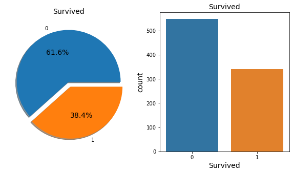
타이타닉호에 탑승한 승객의 생존율은 61.6% 이다.
# 특성별 생존 여부를 piechart로 시각화하기 위한 함수

def pie_chart(feature):
    feature_ratio = train_df[feature].value_counts(sort=False)
    feature_size = feature_ratio.size
    feature_index = feature_ratio.index
    survived = train_df[train_df['Survived'] == 1][feature].value_counts()
    dead = train_df[train_df['Survived'] == 0][feature].value_counts()

    plt.plot(aspect='auto')
    plt.pie(feature_ratio, labels=feature_index, autopct='%1.1f%%')
    plt.title(feature + '\'s ratio in total')
    plt.show()

    for i, idx in enumerate(feature_index):
        plt.subplot(1, feature_size + 1, i + 1, aspect='equal')
        plt.pie([survived[idx], dead[idx]], labels=['Survived', 'Dead'], autopct='%1.1f%%')
        plt.title(str(idx) + '\'s ratio')
    plt.show()
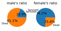
# 성별 별 생존 비율
pie_chart('Sex')
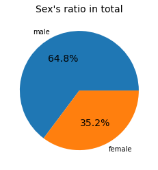
탑승객 중 남자는 64.8%, 여성은 35.2%
- 남자의 생존율 : 18.9%
- 여성의 생존율 : 74.2%
여성의 경우가 생존율이 높았음을 알 수 있다.
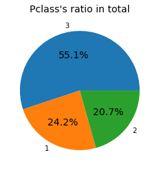
# 객실 등급 Pclass 데이터
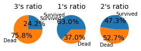
pie_chart('Pclass')
pd.crosstab([train_df['Sex'], train_df['Survived']],
train_df['Pclass'],
margins=True).style.background_gradient(cmap='summer_r')
| Pclass | 1 | 2 | 3 | All | |
|---|---|---|---|---|---|
| Sex | Survived | ||||
| female | 0 | 3 | 6 | 72 | 81 |
| 1 | 91 | 70 | 72 | 233 | |
| male | 0 | 77 | 91 | 300 | 468 |
| 1 | 45 | 17 | 47 | 109 | |
| All | 216 | 184 | 491 | 891 |
탑승권 등급 1등급 24.2% , 2등급 20.7% , 3등급 55.1%로 구성되어 있다.
- 1등급의 생존율: 63.0%
- 2등급의 생존율: 47.3%
- 3등급의 생존율: 24.2%
탑승권 등급이 높을 수록 생존율이 높았음을 알 수 있다.
# 항구의 위치와 연관성
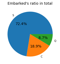
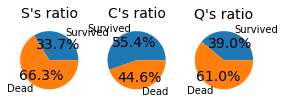
pie_chart("Embarked")
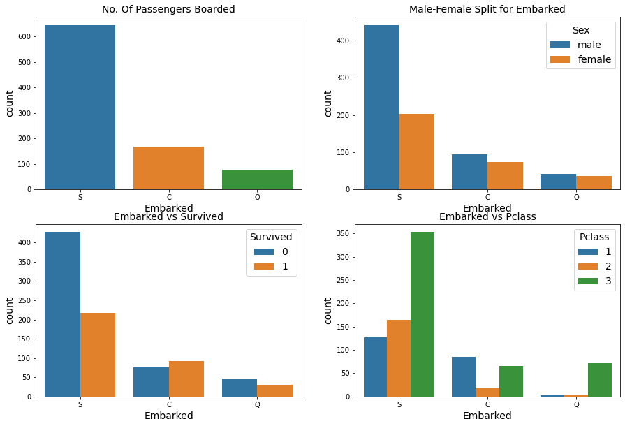
f, ax = plt.subplots(2, 2, figsize=(15,10))
sns.countplot('Embarked', data=train_df, ax=ax[0,0])
ax[0,0].set_title('No. Of Passengers Boarded')
sns.countplot('Embarked', hue='Sex', data=train_df, ax=ax[0,1])
ax[0,1].set_title('Male-Female Split for Embarked')
sns.countplot('Embarked', hue='Survived', data=train_df, ax=ax[1,0])
ax[1,0].set_title('Embarked vs Survived')
sns.countplot('Embarked', hue='Pclass', data=train_df, ax=ax[1,1])
ax[1,1].set_title('Embarked vs Pclass')
plt.show()
-
항구별 탑승자 비율 : 절반 이상의 사람이 S항구를 통해 입항한 것을 볼 수 있음
-
항구별 탑승자 성별 : S항구를 통해 들어온 사람들의 성별은 남성이 많은 수를 차지함
-
항구별 생존율: 많은 사람이 탄 만큼 S항구의 생존율이 낮음, C항구의 생존률이 높음
-
항구별 탑승권 등급 : S항구와 Q항구는 3등급객실의 비율이 높으며, C는 1등급객실의 비율이 높음. C항구가 부유한 계층이 사는 지역임을 유추할 수 있음.
# 특성별 생존 여부를 barchart로 시각화하기 위한 함수
def bar_chart(feature):
    survived = train_df[train_df["Survived"] == 1][feature].value_counts()
    dead = train_df[train_df["Survived"] == 0][feature].value_counts()
    df = pd.DataFrame([survived, dead])
    df.index = ["Survived", "Dead"]
    df.plot(kind='bar', stacked=True, figsize=(10,5))
# SibSp 시각화
sibsp_ratio = train_df["SibSp"].value_counts()
plt.pie(sibsp_ratio, labels=sibsp_ratio.index, autopct='%1.1f%%')
plt.title('SibSp\'s ratio')
plt.show()
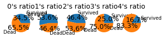
survived= train_df[train_df['Survived'] == 1]["SibSp"].value_counts()
dead = train_df[train_df['Survived'] == 0]["SibSp"].value_counts()
for i, index in enumerate(survived.index):
plt.subplot(1, survived.size+1, i+1, aspect='equal')
plt.pie([survived[index], dead[index]], labels=["Survived", "Dead"], autopct='%1.1f%%')
plt.title(str(index) + '\'s ratio')
plt.show()
bar_chart("SibSp")
train_df["SibSp"].value_counts()
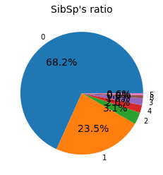
0    608
1    209
2     28
4     18
3     16
8      7
5      5
Name: SibSp, dtype: int64
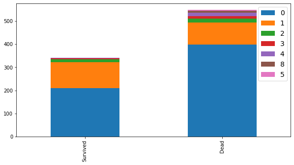
형제 또는 배우자가 동승하지 않은 경우는 68.2%, 동승한 경우는 31.8%이다.
동승자의 수가 1명 또는 2명인 경우가 생존율이 제일 높았다.
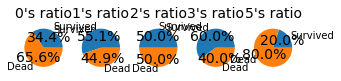
# Parch 시각화
parch_ratio = train_df["Parch"].value_counts()
plt.pie(parch_ratio, labels=parch_ratio.index, autopct='%1.1f%%')
plt.title('Parch\'s ratio')
plt.show()
survived= train_df[train_df['Survived'] == 1]["Parch"].value_counts()
dead = train_df[train_df['Survived'] == 0]["Parch"].value_counts()

for i, index in enumerate(survived.index):
    plt.subplot(1, survived.size+1, i+1, aspect='equal')
    plt.pie([survived[index], dead[index]], labels=["Survived", "Dead"], autopct='%1.1f%%')
    plt.title(str(index) + '\'s ratio')
plt.show()
bar_chart("Parch")
train_df["Parch"].value_counts()
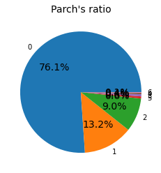
0    678
1    118
2     80
5      5
3      5
4      4
6      1
Name: Parch, dtype: int64
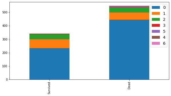
부모 또는 자녀가 동승하지 않은 경우는 76.1%이며, 동승한 경우는 23.9%이다.
동승자가 없는 탑승객보다 1명 ~ 3명까지 동승한 탑승객의 생존율이 높았다.
데이터를 시각화해본 결과로 알아본 데이터 특성간 유의한 정보는 남자보단 여자, 부유한 계층일 수록 생존율이 높은 것이다.
이를 데이터 전처리 하는데 사용하도록 한다.
데이터 전처리
# 결측치 확인
print(train_df.isnull().sum())
print()
print(test_df.isnull().sum())
PassengerId      0
Survived         0
Pclass           0
Name             0
Sex              0
Age            177
SibSp            0
Parch            0
Ticket           0
Fare             0
Cabin          687
Embarked         2
dtype: int64

PassengerId      0
Pclass           0
Name             0
Sex              0
Age             86
SibSp            0
Parch            0
Ticket           0
Fare             1
Cabin          327
Embarked         0
dtype: int64
훈련셋에는 나이와 카빈, 항구 값에 누락치가 있고, 테스트 셋에는 나이, Fare, 카빈에 누락치가 있다.
train_df['Name'].head()
0                              Braund, Mr. Owen Harris
1    Cumings, Mrs. John Bradley (Florence Briggs Th...
2                               Heikkinen, Miss. Laina
3         Futrelle, Mrs. Jacques Heath (Lily May Peel)
4                             Allen, Mr. William Henry
Name: Name, dtype: object
전처리 과정
-
Name 특성에서 승객들 이름 앞에 title을 새로운 특성으로 만들어 사용한다.
-
Embarked 특성은 결측치를 최빈값으로 채운다.
-
Age 특성은 결측치는 평균으로 대체한 후 연속 데이터를 범주 데이터로 변환한다.
-
Fare 특성는 Pclass와 연관이 있음으로, Fare 특성이 결측된 값을 Pclass 평균값으로 넣어 후, 범주 데이터로 변환한다.
-
나머지 PassengerId, Name, Ticket, Cabin 특성은 drop한다.
-
범주형 데이터를
OneHotEncoding을 통해 정수로 변환한다.
1.
Name 특성을 보면 이름과 성 사에 Mr. Mrs. Dr. 등의 타이틀이 붙는다. 이 타이틀을 통해 성별 또는 신분, 직업을 예측할 수 있음으로 Title이라는 새로운 특성을 만들어 사용한다.
# 1
def title_pipeline(titanic):
    titanic['Title'] = titanic.Name.str.extract(' ([A-Za-z]+)\.')
    titanic['Title'] = titanic['Title'].replace(['Capt', 'Col', 'Countess', 'Don','Dona', 'Dr', 'Jonkheer',
                                                'Lady','Major', 'Rev', 'Sir'], 'Other')
    titanic['Title'] = titanic['Title'].replace('Mlle', 'Miss')
    titanic['Title'] = titanic['Title'].replace('Mme', 'Mrs')
    titanic['Title'] = titanic['Title'].replace('Ms', 'Miss')
    titanic['Title'] = titanic['Title'].astype(str)
    return titanic
([A-Za-z]+)\.' 는 정규표현식으로 공백으로 시작하고, .으로 끝나는 문자열을 추출할 때 사용한다.
title_test = train_df.copy()
title_test = title_pipeline(title_test)
print(title_test["Title"].value_counts())
print(title_test[['Title', 'Survived']].groupby(['Title'], as_index=False).mean())
Mr        517
Miss      185
Mrs       126
Master     40
Other      23
Name: Title, dtype: int64
    Title  Survived
0  Master  0.575000
1    Miss  0.702703
2      Mr  0.156673
3     Mrs  0.793651
4   Other  0.347826
2.
# 2
def embarked_pipeline(titanic):
    titanic['Embarked'] = titanic['Embarked'].fillna('S')
    titanic['Embarked'] = titanic['Embarked'].astype(str)
    return titanic
3.
# 5
def age_pipeline(titanic):
    titanic['Age'].fillna(titanic['Age'].mean(), inplace=True)
    titanic.loc[ titanic['Age'] <= 16, 'Age'] = 0
    titanic.loc[ (titanic['Age'] > 16) & (titanic['Age'] <= 32), 'Age'] = 1
    titanic.loc[ (titanic['Age'] > 32) & (titanic['Age'] <= 48), 'Age'] = 2
    titanic.loc[ (titanic['Age'] > 48) & (titanic['Age'] <= 64), 'Age'] = 3
    titanic.loc[ titanic['Age'] > 64, 'Age'] = 4
    titanic['Age'] = titanic['Age'].map({ 0: 'Child', 1: 'Young', 2: 'Middle', 3: 'Prime', 4: 'Old'}).astype(str)
    return titanic
4.
# 4
def fare_pipeline(titanic):
    titanic['Fare'] = titanic['Fare'].fillna(13.675)
    titanic.loc[ titanic['Fare'] <= 7.854, 'Fare'] = 0
    titanic.loc[ (titanic['Fare'] > 7.854) & (titanic['Fare'] <= 10.5), 'Fare'] = 1
    titanic.loc[ (titanic['Fare'] > 10.5) & (titanic['Fare'] <= 21.679), 'Fare'] = 2
    titanic.loc[ (titanic['Fare'] > 21.679) & (titanic['Fare'] <= 39.688), 'Fare'] = 3
    titanic.loc[ titanic['Fare'] > 39.688, 'Fare'] = 4
    titanic['Fare'] = titanic['Fare'].astype(int)
    return titanic
5.
# 5
def drop_pipeline(titanic):
    features_drop = ["PassengerId","Name", "Ticket", "Cabin"]
    titanic_prepared = titanic.drop(features_drop, axis=1)
    return titanic_prepared
6.
# 6.
from sklearn.compose import ColumnTransformer, make_column_selector
from sklearn.preprocessing import OneHotEncoder, FunctionTransformer, StandardScaler

def cat_pipeline():
    return ColumnTransformer([("cat", OneHotEncoder(handle_unknown='ignore'), make_column_selector(dtype_include=object))],
                                         remainder = 'passthrough')
전처리 파이프라인
# 전처리 파이프라인
from sklearn.pipeline import Pipeline
from sklearn import set_config
set_config(display='diagram')

preprocessing = Pipeline([("title_preprocessing", FunctionTransformer(title_pipeline)),
                         ("embarked_preprocessing", FunctionTransformer(embarked_pipeline)),
                         ("age_preprocessing", FunctionTransformer(age_pipeline)),
                         ("fare_preprocessing", FunctionTransformer(fare_pipeline)),
                         ("drop_preprocessing", FunctionTransformer(drop_pipeline)),
                         ("cat_preprocessing", cat_pipeline())])
훈련셋 전처리하기
titanic_label : 타이타닉 탑승객의 생존여부 정보
titanic : 전처리할 특성
titanic_prepare = train_df.copy()
titanic_label = titanic_prepare['Survived'].copy()
titanic = titanic_prepare.drop("Survived", axis=1)
titanic = preprocessing.fit_transform(titanic)
print(titanic)
print(titanic.shape)
[[0. 1. 0. ... 1. 0. 0.]
 [1. 0. 0. ... 1. 0. 4.]
 [1. 0. 0. ... 0. 0. 1.]
 ...
 [1. 0. 0. ... 1. 2. 3.]
 [0. 1. 0. ... 0. 0. 3.]
 [0. 1. 0. ... 0. 0. 0.]]
(891, 19)
테스트셋 전처리하기
test_set = test_df.copy()
test_set = preprocessing.fit_transform(test_set)
test_set.shape
(418, 19)
모델 학습과 훈련
모델 학습과 평가에 필요한 pipeline을 만들어 훈련된 결과를 평가한다.
평가예정 모델
LogisticRegression선형회귀모델SVCSVC 모델KNeighborsClassifierRandomForestClassifier랜덤포레스트 모델GaussianNB
평가 : 교차검증
from sklearn.linear_model import LogisticRegression
from sklearn.svm import SVC
from sklearn.neighbors import KNeighborsClassifier
from sklearn.ensemble import RandomForestClassifier
from sklearn.naive_bayes import GaussianNB
from sklearn.model_selection import cross_val_score
from sklearn.utils import shuffle

# 데이터 셔플
titanic, titanic_label = shuffle(titanic, titanic_label, random_state=42)

# 모델 학습과 평가에 대한 pipeline
def train_and_test(model):
    model.fit(titanic, titanic_label)
    prediction = model.predict(test_set)

    accuracy = cross_val_score(model, titanic, titanic_label, cv=10)
    accuracy = accuracy.mean()
    print(f"Accuracy : {accuracy} %")
    return prediction
log_pred = train_and_test(LogisticRegression())
svm_pred = train_and_test(SVC())
knn_pred_4 = train_and_test(KNeighborsClassifier(n_neighbors = 4))
rf_pred = train_and_test(RandomForestClassifier(n_estimators=100))
nb_pred = train_and_test(GaussianNB())
Accuracy : 0.8215480649188514 %
Accuracy : 0.8316354556803995 %
Accuracy : 0.8181772784019975 %
Accuracy : 0.8102996254681647 %
Accuracy : 0.7789013732833958 %
제출
교차검증을 통해 83.16%를 보인 SVC 모델을 채택해서 제출한다.
제출은 캐글 사이트에서 Submit Predictions에서 제출할 수 있으며, 캐글 노트북에서 작성할 경우 예측한 파일 이름을 submission.csv으로 해야한다.
submission = pd.DataFrame({
    "PassengerId": test_df["PassengerId"],
    "Survived": svm_pred
})

submission.to_csv('submission.csv', index=False)

채점 결과 교차검증에서 정확도 보다 낮은 77.99%가 나왔다.
개선 해야할 점
GridSearchCV 또는 RandomizedSearchCV 를 통해 더 많은 모델과 하이퍼파라미터 설정을 비교하면 좋아질 것 같다.
Leave a comment