[MachineLearning] 요리지역분류(2)
포스팅에 앞서 본 내용은 ML-For-Beginners를 요약 정리하며 공부한 것임을 알려드립니다.
머신러닝 - 음식지역 분류
이번 포스팅에서는 이전포스팅에서 전처리한 데이터를 불러온 후 문제를 해결한다.
문제: 사용된 재료를 가지고 요리의 지역을 분류한다.
# 데이터 불러오기
import pandas as pd
import numpy as np

cuisines_df = pd.read_csv('./datasets/classifier/cleaned_cuisines.csv')
cuisines_df
| Unnamed: 0 | cuisine | almond | angelica | anise | anise_seed | apple | apple_brandy | apricot | armagnac | ... | whiskey | white_bread | white_wine | whole_grain_wheat_flour | wine | wood | yam | yeast | yogurt | zucchini | |
|---|---|---|---|---|---|---|---|---|---|---|---|---|---|---|---|---|---|---|---|---|---|
| 0 | 0 | indian | 0 | 0 | 0 | 0 | 0 | 0 | 0 | 0 | ... | 0 | 0 | 0 | 0 | 0 | 0 | 0 | 0 | 0 | 0 |
| 1 | 1 | indian | 1 | 0 | 0 | 0 | 0 | 0 | 0 | 0 | ... | 0 | 0 | 0 | 0 | 0 | 0 | 0 | 0 | 0 | 0 |
| 2 | 2 | indian | 0 | 0 | 0 | 0 | 0 | 0 | 0 | 0 | ... | 0 | 0 | 0 | 0 | 0 | 0 | 0 | 0 | 0 | 0 |
| 3 | 3 | indian | 0 | 0 | 0 | 0 | 0 | 0 | 0 | 0 | ... | 0 | 0 | 0 | 0 | 0 | 0 | 0 | 0 | 0 | 0 |
| 4 | 4 | indian | 0 | 0 | 0 | 0 | 0 | 0 | 0 | 0 | ... | 0 | 0 | 0 | 0 | 0 | 0 | 0 | 0 | 1 | 0 |
| ... | ... | ... | ... | ... | ... | ... | ... | ... | ... | ... | ... | ... | ... | ... | ... | ... | ... | ... | ... | ... | ... |
| 3990 | 3990 | thai | 0 | 0 | 0 | 0 | 0 | 0 | 0 | 0 | ... | 0 | 0 | 0 | 0 | 0 | 0 | 0 | 0 | 0 | 0 |
| 3991 | 3991 | thai | 0 | 0 | 0 | 0 | 0 | 0 | 0 | 0 | ... | 0 | 0 | 0 | 0 | 0 | 0 | 0 | 0 | 0 | 0 |
| 3992 | 3992 | thai | 0 | 0 | 0 | 0 | 0 | 0 | 0 | 0 | ... | 0 | 0 | 0 | 0 | 0 | 0 | 0 | 0 | 0 | 0 |
| 3993 | 3993 | thai | 0 | 0 | 0 | 0 | 0 | 0 | 0 | 0 | ... | 0 | 0 | 0 | 0 | 0 | 0 | 0 | 0 | 0 | 0 |
| 3994 | 3994 | thai | 0 | 0 | 0 | 0 | 0 | 0 | 0 | 0 | ... | 0 | 0 | 0 | 0 | 0 | 0 | 0 | 0 | 0 | 0 |
3995 rows × 382 columns
훈련을 시키기 위해 불러온 데이터를 특성(사용된 재료)과 지도학습의 라벨(지역)로 나눈다.
# 특성과 라벨을 나눈다.
cuisines_feature_df = cuisines_df.drop(['Unnamed: 0', 'cuisine'], axis=1)
cuisines_label_df = cuisines_df['cuisine']
cuisines_feature_df.head()
| almond | angelica | anise | anise_seed | apple | apple_brandy | apricot | armagnac | artemisia | artichoke | ... | whiskey | white_bread | white_wine | whole_grain_wheat_flour | wine | wood | yam | yeast | yogurt | zucchini | |
|---|---|---|---|---|---|---|---|---|---|---|---|---|---|---|---|---|---|---|---|---|---|
| 0 | 0 | 0 | 0 | 0 | 0 | 0 | 0 | 0 | 0 | 0 | ... | 0 | 0 | 0 | 0 | 0 | 0 | 0 | 0 | 0 | 0 |
| 1 | 1 | 0 | 0 | 0 | 0 | 0 | 0 | 0 | 0 | 0 | ... | 0 | 0 | 0 | 0 | 0 | 0 | 0 | 0 | 0 | 0 |
| 2 | 0 | 0 | 0 | 0 | 0 | 0 | 0 | 0 | 0 | 0 | ... | 0 | 0 | 0 | 0 | 0 | 0 | 0 | 0 | 0 | 0 |
| 3 | 0 | 0 | 0 | 0 | 0 | 0 | 0 | 0 | 0 | 0 | ... | 0 | 0 | 0 | 0 | 0 | 0 | 0 | 0 | 0 | 0 |
| 4 | 0 | 0 | 0 | 0 | 0 | 0 | 0 | 0 | 0 | 0 | ... | 0 | 0 | 0 | 0 | 0 | 0 | 0 | 0 | 1 | 0 |
5 rows × 380 columns
cuisines_label_df.head()
0    indian
1    indian
2    indian
3    indian
4    indian
Name: cuisine, dtype: object
모델 선택에 관한 이론
정처리된 데이터를 가지고 훈련을 진행한다.
사이킷런은 다양한 분류 알고리즘을 이용한 분류기를 제공하며 분류 알고리즘은 대략 아래와 같다.
- Linear Models
- Support Vector Machines
- Stochastic Gradient Descent
- Nearest Neighbors
- Gaussian Processes
- Decision Trees
- Ensemble methods (voting Classifier)
- Multiclass and multioutput algorithms (multiclass and multilabel classification, multiclass-multioutput classification)
또한 neural networks 를 통해 데이터를 분류할 수 있지만 이번 포스팅에서는 다루지 않겠습니다.
분류기를 선택하는 방법은 여러 가지를 실행하고 좋은 결과를 찾는 것이 일반적인 방법이다.
사이킷런에서 10가지 다른 예측기에 따른 데이터 분류를 시각화 해서 보여준다.
- KNeighbors
- SVC의 2가지 커널방식(linear, rbf)
- GaussianProcessClassifier
- DecisionTreeClassifier
- RandomForestClassifier
- MLPClassifier
- AdaBoostClassifier
- GaussianNB
- QuadraticDiscrinationAnalysis,
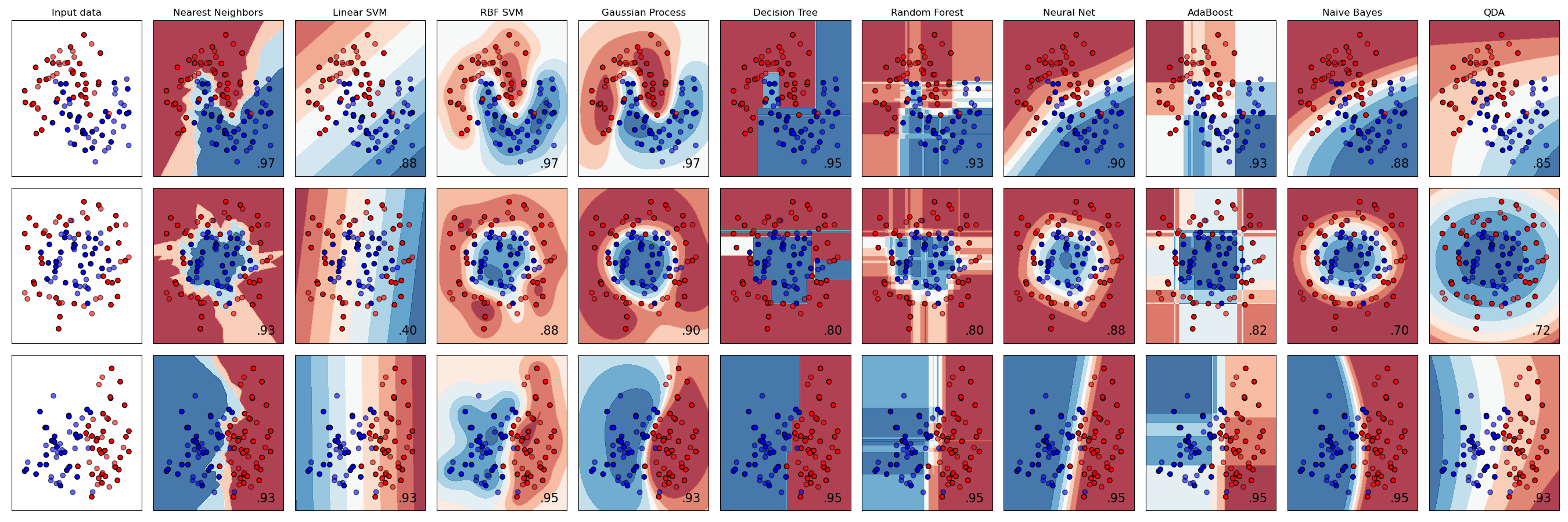
출처: Scikit-learn.Classifier comparison
다중 클래스 분류
다중 클래스 분류를 하기 위해 여러가지 선택사항이 있다.
| 선택사항 | 특징 |
|---|---|
| 다중클래스 Logistic Regression | 빠른 훈련시간, 선형모델 |
| 다중클래스 Decision Forest | 높은 정확도, 빠른 훈련시간 |
| 다중클래스 Neural Network | 높은 정확도, 긴 훈련시간 |
| One-vs-All 다중클래스 | 이진분류기를 통한 다중클래스 분류 |
| 다중클래스 Boosted Decision Tree | Non-parametric, 빠른 훈련시간, scalable |
선택사항에 대한 설명
- 결정트리 모델 또는 논리회귀 모델은 사용가능하다.
- 다중클래스 Neural Network 는 좋은 성능을 보이지만 우리가 수행해야될 과제에 비해 너무 무겁다.
- Boosted Decision Tree는 비모수 과제에 적합하며 순위를 만들기 위해 만들어진 모델이므로 우리 과제에는 유용하지 않다.
데이터 분류를 하기 위해 사이킷런 패키지에서 제공하는 예측기를 사용할 것이며 분류모델을 다중클래스 분류로 사용하기 위해 하이퍼파라미터 설정이 필요한 모델들이 있다.
LogisticRegression 예측기를 사용하는 경우 하이퍼파라미터 multi_class와 solver를 설정해야한다.
multi_class='ovr': one-vs-rest 방식multi_class='multinomial': multinomial로 설정한 경우
현재 solver는 ‘lbfgs’, ‘sag’, ‘saga’, ‘newton-cg’만 지원한다.
사이킷런 sklearn.linear_model.LogisticRegression에서 solver에 따라 지원하는 규제를 알 수 있다.
| solvers | |||||
|---|---|---|---|---|---|
| Penalties | ‘liblinear’ | ‘lbfgs’ | ‘newton-cg’ | ‘sag’ | ‘saga’ |
| Multinomial + L2 penalty | X | O | O | O | O |
| OVR + L2 penalty | O | O | O | O | O |
| Multinomial + L1 penalty | X | X | X | X | O |
| OVR + L1 penalty | O | X | X | X | O |
| Elastic-Net | X | X | X | X | O |
| none | X | O | O | O | O |
| Behaviors | |||||
| Penalize the intercept (bad) | O | X | X | X | X |
| Faster for large datasets | X | X | X | O | O |
| Robust to unscaled datasets | O | O | O | X | X |
데이터 셋 나누기
sklearn 패키지의 train_test_split()을 통해 훈련셋과 테스트셋으로 나눈다.
테스트셋의 크기는 전체 테이터셋의 30%로 한다.
from sklearn.model_selection import train_test_split

X_train, X_test, y_train, y_test = train_test_split(cuisines_feature_df, cuisines_label_df, test_size=0.3, random_state=42)
LogisticRegression
sklearn의 LogisticRegression 예측기를 사용하여 다중클래스 분류를 실행한다.
1.multi_class='ovr' , solve='liblinear'로 하이퍼 파라미터를 설정한 후 훈련시켰을 때 정확도
from sklearn.linear_model import LogisticRegression

log_clf = LogisticRegression(multi_class='ovr', solver='liblinear')
model = log_clf.fit(X_train, np.ravel(y_train))

accuracy = model.score(X_test, y_test)
print(f"Accuracy is {accuracy}")
Accuracy is 0.7973311092577148
2.multi_class='multinomial' , solver='lbfgs'로 하이퍼 파라미터를 설정한 후 훈련시켰을 때 정확도.
solver의 기본값이 ‘lbfgs’이므로 설정하지 않고 훈련시킨다.
log_clf = LogisticRegression(multi_class='multinomial')
model = log_clf.fit(X_train, np.ravel(y_train))

accuracy = model.score(X_test, y_test)
print(f"Accuracy is {accuracy}")
Accuracy is 0.8031693077564637
1(multi_class='ovr' , solve='liblinear')과 2(multi_class='multinomial' , solver='lbfgs')는 둘다 대략 80%로 비슷한 정확도를 보이지만, 2번의 경우가 정확도가 미세하게 더 높은 것을 볼 수 있다.
테스트셋 처음 50개의 샘플을 각 클래스에 대해 예측함수의 결과를 확인한다.
test = X_test.iloc[50].values.reshape(-1, 1).T
proba = model.predict_proba(test)
classes = model.classes_
resultdf = pd.DataFrame(data=proba, columns=classes)

topPrediction = resultdf.T.sort_values(by=[0], ascending=[False])
topPrediction.head()
| 0 | |
|---|---|
| indian | 0.707395 |
| thai | 0.284868 |
| japanese | 0.006503 |
| chinese | 0.001166 |
| korean | 0.000068 |
인도음식에 대한 예측이 가장 좋은 확률을 보인다.
분류의 성능을 더 자세히 평가하기 위해서 classification_report 메서드를 통해 정밀도, 재현율, f1점수(정밀도와 재현율의 조화평균)을 확인한다.
from sklearn.metrics import accuracy_score, precision_score,\
  confusion_matrix, classification_report, precision_recall_curve

y_pred = model.predict(X_test)
print(classification_report(y_test,y_pred))
              precision    recall  f1-score   support

     chinese       0.75      0.69      0.72       236
      indian       0.90      0.91      0.90       245
    japanese       0.76      0.81      0.78       231
      korean       0.83      0.77      0.80       242
        thai       0.77      0.83      0.80       245

    accuracy                           0.80      1199
   macro avg       0.80      0.80      0.80      1199
weighted avg       0.80      0.80      0.80      1199
여러 모델을 훈련시킨 후 훈련선택
이제 위에서 나눈 훈련셋과 테스트셋을 가지고 여러 예측기를 사용해 음식의 종류를 분류한다. 사용할 모델은 아래와 같다.
- LinearSVC
- SVC
- LogisticRegression
- KNeighborsClassifier
- RandomForestClassifier
Linear kernerl SVC
서포트 벡터 군집화는 kernel='linear'로 설정된 서포즈 벡터 머신이다.
C: 규제 정도를 말하며 양수C0에 가까울 수록 규제가 강해진다.probability: bool값을 받으며 확률 추정를 사용하는지 여부를 설정한다.fit을 실행하기 전에 설정해야 하며, True로 설정하면 5-fold 교차검증을 한다. default값은 False이다.random_state를 42로 설정한다.
K-Neighbors classifier
지도학습과 비지도학습에서 사용하는 머신러닝 메서드로 k개의 포인트로 군집화를 시킨다.
n_neighbors: neighbors의 개수p: 거리함수이다. p=1이면 맨해튼거리, p=2이면 유클리디안거리이다.
Support Vector Classifier
서포트 벡터 머신 중 하나로 분류와 회귀의 과제를 해결할 수 있다.
C: 규제 정도, 숫자가 커질수록 규제강도 낮아짐kernel: 알고리즘에 사용되는 커널의 타입을 결정 default: ‘rbf’linear: 선형poly: 다항식,degree와 같이씀rbf: 가우시안 RBFgamma를 통해 가까운 샘플를 선호하는 정도를 설정한다.
RandomForestClassifier
n_estimator개의 결정트리 모델을 사용하여 훈련한다.
AdaBoostClassifier
분류기를 데이터셋에 맞춘 다음 복사한 분류기에 같은 데이터셋을 학습시킨다. 잘못 분류된 샘플의 파라미터를 다음 분류기가 수정하도록 조정한다.
# 필요한 모델 import
from sklearn.neighbors import KNeighborsClassifier
from sklearn.linear_model import LogisticRegression
from sklearn.svm import SVC, LinearSVC
from sklearn.ensemble import RandomForestClassifier, AdaBoostClassifier
from sklearn.model_selection import train_test_split, cross_val_score
from sklearn.metrics import accuracy_score,precision_score,confusion_matrix,classification_report, precision_recall_curve
import numpy as np
C = 10

classifiers = {
    'Linear SVC': LinearSVC(C=C, random_state=42),
    'Linear kernel SVC': SVC(kernel='linear', probability=True, random_state=42),
    'KNN classifier': KNeighborsClassifier(C),
    'SVC': SVC(random_state=42),
    'RFST': RandomForestClassifier(n_estimators=100, random_state=42),
    'ADA': AdaBoostClassifier(n_estimators=100, random_state=42)
}
n_classifiers = len(classifiers)

for index, (name, classifiers) in enumerate(classifiers.items()):
    classifiers.fit(X_train, np.ravel(y_train))

    y_pred = classifiers.predict(X_test)
    accuracy = accuracy_score(y_test, y_pred)
    print(f"Accuracy for {name} : {accuracy * 100:.2f}")
Accuracy for Linear SVC : 79.73
Accuracy for Linear kernel SVC : 78.90
Accuracy for KNN classifier : 69.31
Accuracy for SVC : 81.23
Accuracy for RFST : 81.98
Accuracy for ADA : 67.14
랜덤포레스트 모델이 81.98 %로 테스트셋을 평가한 정확도가 가장 높았으며 classification_report()함수를 통해 분류기의 성능을 확인하는 것은 아래와 같다.
rf_clf = RandomForestClassifier(n_estimators=100, random_state=42)
rf_clf.fit(X_train, np.ravel(y_train))
y_pred = rf_clf.predict(X_test)

print(classification_report(y_test, y_pred))
              precision    recall  f1-score   support

     chinese       0.74      0.79      0.76       236
      indian       0.88      0.92      0.90       245
    japanese       0.82      0.79      0.80       231
      korean       0.87      0.74      0.80       242
        thai       0.79      0.86      0.82       245

    accuracy                           0.82      1199
   macro avg       0.82      0.82      0.82      1199
weighted avg       0.82      0.82      0.82      1199
랜덤포레스트분류기로 인도음식을 분류할 때, 정밀도와 재현율이 가장 높다.
훈련된 모델 onnx파일로 다운
skl2onnx 모듈을 사용하여 훈련된 사이킷런 모델을 Onnx포멧으로 저장한다.
skl2onnx 모듈을 다운 받기 위해 아래의 명령어를 프롬포트에 입력한다.
pip install skl2onnx
구글코랩이나 주피터노트북의 경우
!pip install skl2onnx
from skl2onnx import convert_sklearn
from skl2onnx.common.data_types import FloatTensorType

initial_types = [('float_input', FloatTensorType([None, 380]))]
options = {id(rf_clf): {'nocl':False, 'zipmap': False}}

onx = convert_sklearn(rf_clf, initial_types=initial_types, options=options)
with open("./model.onnx", "wb") as f:
    f.write(onx.SerializeToString())
NOTE: 변환스크립트에 option을 전달할 수 있다. 위 경우에 ‘nocl’:False, ‘zipmap’: False을 옵션으로 전달했다.
분류모델이기 때문에 dict의 list를 생성하는 ZipMap은 필수가 아닙니다.
‘nocl’은 모델의 클래스정보를 저장할 것인가 유무이며 ‘nocl’:True로 설정하면 클래스정보를 저장하지 않아 모델의 크기를 줄일 수 있습니다.
notebook이 실행되는 위치에 onnx 파일이 생성된 것을 볼 수 있다.
다음 포스팅에서는 onnx로 다운받은 파일을 통해 재료를 입력하면 어느나라의 음식을 만들 것인지 판단하는 웹서비스를 구현한다.
Leave a comment