[MachineLearning] 요리지역분류(1)

포스팅에 앞서 본 내용은 ML-For-Beginners를 요약 정리하며 공부한 것임을 알려드립니다.

머신러닝 - 음식지역 분류

소개

머신러닝 기법 중 분류에 대해서 설명한다.

분류는 지도학습에서 주로 사용되며 회귀와 많은 공통점이 있다.

• 선형회귀: 변수들 사이의 관계를 통해 타겟을 예측한다. 예시: 11월,12월의 호박값 예측

• 논리회귀: 두개로 나눠진 범주를 예측한다. 예시: 호박이 노란가 안노란가

Note: 지도학습은 훈련 데이터에 레이블이라는 답을 표기하여 레이블을 맞추도록 유도하는 학습을 가르킨다.

분류는 크게 이진분류와 다중클래스 분류로 나뉜다.
메일의 분류

• 이진분류: 메일이 스팸메일인가 아닌가?
• 다중클래스 분류: 광고메일, 업무메일, 일상메일 나누기

분류는 데이터의 라벨 또는 클래스를 결정하는 다양한 알고리즘을 사용한다. 이 포스팅에서는 다양한 분류알고리즘을 통해 인도와 아시아의 요리를 분류할 것이다.

강의에서 사용할 요리 데이터는 다중클래스를 가진 데이터로 여러 지역의 요리로 되어있다.

분류는 Scikit-learn 패키지에서 제공하는 다양한 알고리즘을 사용할 것이다.

데이터 전처리

첫번째로 사이킷런 패키지의 imblearn를 설치해야한다.

윈도우 기준 프롬포트에 아래의 명령어를 통해 설치를 한다.
pip install imblearn
구글코랩이나 주피터노트북을 사용한다면
!pip install imblearn
을 사용한다.

데이터 시각화

데이터 시각화와 데이터를 불러오기 위한 코드를 작성한다.

import pandas as pd
import matplotlib.pyplot as plt
import matplotlib as mpl
import numpy as np
from imblearn.over_sampling import SMOTE

# 데이터 불러오기
datapath = "https://raw.githubusercontent.com/codingalzi/ML-For-Beginners/main/4-Classification/data/cuisines.csv"
df = pd.read_csv(datapath)
# 데이터 shape 확인
df

	Unnamed: 0	cuisine	almond	angelica	anise	anise_seed	apple	apple_brandy	apricot	armagnac	...	whiskey	white_bread	white_wine	whole_grain_wheat_flour	wine	wood	yam	yeast	yogurt	zucchini
0	65	indian	0	0	0	0	0	0	0	0	...	0	0	0	0	0	0	0	0	0	0
1	66	indian	1	0	0	0	0	0	0	0	...	0	0	0	0	0	0	0	0	0	0
2	67	indian	0	0	0	0	0	0	0	0	...	0	0	0	0	0	0	0	0	0	0
3	68	indian	0	0	0	0	0	0	0	0	...	0	0	0	0	0	0	0	0	0	0
4	69	indian	0	0	0	0	0	0	0	0	...	0	0	0	0	0	0	0	0	1	0
...	...	...	...	...	...	...	...	...	...	...	...	...	...	...	...	...	...	...	...	...	...
2443	57686	japanese	0	0	0	0	0	0	0	0	...	0	0	0	0	0	0	0	0	0	0
2444	57687	japanese	0	0	0	0	0	0	0	0	...	0	0	0	0	0	0	0	0	0	0
2445	57688	japanese	0	0	0	0	0	0	0	0	...	0	0	0	0	0	0	0	0	0	0
2446	57689	japanese	0	0	0	0	0	0	0	0	...	0	0	0	0	0	0	0	0	0	0
2447	57690	japanese	0	0	0	0	0	0	0	0	...	0	0	0	0	0	0	0	0	0	0

2448 rows × 385 columns

# info()
df.info()

<class 'pandas.core.frame.DataFrame'>
RangeIndex: 2448 entries, 0 to 2447
Columns: 385 entries, Unnamed: 0 to zucchini
dtypes: int64(384), object(1)
memory usage: 7.2+ MB

총 2448개의 샘플을 가지고 385개의 특성을 가진다.

cuisine : 요리의 지역 (클래스)

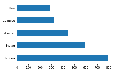
데이터의 클래스를 가로 바그래프로 시각화 (barh())

df.cuisine.value_counts().plot.barh()

요리데이터의 나라별 데이터 shape

thai_df = df[(df.cuisine == "thai")]
japanese_df = df[(df.cuisine == "japanese")]
chinese_df = df[(df.cuisine == "chinese")]
indian_df = df[(df.cuisine == "indian")]
korean_df = df[(df.cuisine == "korean")]

print(f'thai df: {thai_df.shape}')
print(f'japanese df: {japanese_df.shape}')
print(f'chinese df: {chinese_df.shape}')
print(f'indian df: {indian_df.shape}')
print(f'korean df: {korean_df.shape}')

thai df: (289, 385)
japanese df: (320, 385)
chinese df: (442, 385)
indian df: (598, 385)
korean df: (799, 385)

한국 요리가 799개의 샘플을 가지고 있고 가장 적은 것은 태국 요리가 289개의 샘플을 가지고 있다.
이처럼 요리의 지역이 고르게 분포하고 있지 않기 때문에 데이터 분포를 고르게 만들어야 한다.

또한 데이터를 파악해 지역별 요리의 일반적인 재료가 무엇인지 알아봐야한다.
재료가 여러지역에 똑같이 많이 들어간다면 분류를 훈련하는데 필요없는 특성으로 혼동을 주는 데이터 특성을 정리해야한다.

# 재료를 보여주는 데이터프래임을 생성하는 함수
# 도움되지 않는 특성을 제거하고, 재료가 많이 들어간 순으로 정렬
def create_ingredient_df(df):
    ingredient_df = df.T.drop(['cuisine', 'Unnamed: 0']).sum(axis=1).to_frame('value')
    ingredient_df = ingredient_df[(ingredient_df.T != 0).any()]
    ingredient_df = ingredient_df.sort_values(by='value', ascending=False, inplace=False)
    return ingredient_df

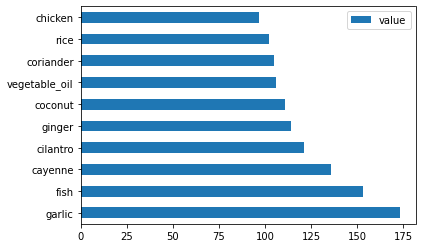
# 태국 요리의 재료 중 많이 들어간 상위 10개
# 바그래프으로 시각화
thai_ingredient_df = create_ingredient_df(thai_df)
thai_ingredient_df.head(10).plot.barh()

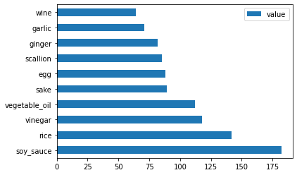
# 일본 요리의 재료 중 많이 들어간 상위 10개
# 바그래프으로 시각화
japanese_ingredient_df = create_ingredient_df(japanese_df)
japanese_ingredient_df.head(10).plot.barh()

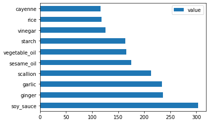
# 중국 요리의 재료 중 많이 들어간 상위 10개
# 바그래프으로 시각화
chinese_ingredient_df = create_ingredient_df(chinese_df)
chinese_ingredient_df.head(10).plot.barh()

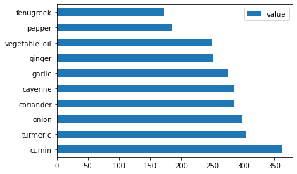
# 인도 요리의 재료 중 많이 들어간 상위 10개
# 바그래프으로 시각화
indian_ingredient_df = create_ingredient_df(indian_df)
indian_ingredient_df.head(10).plot.barh()

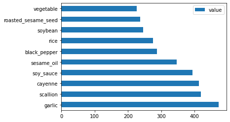
# 한국 요리의 재료 중 많이 들어간 상위 10개
# 바그래프으로 시각화
korean_ingredient_df = create_ingredient_df(korean_df)
korean_ingredient_df.head(10).plot.barh()

confusion_f = (korean_ingredient_df.head(20).index & japanese_ingredient_df.head(20).index 
              & indian_ingredient_df.head(20).index & chinese_ingredient_df.head(20).index
              & thai_ingredient_df.head(20).index)
confusion_f

Index(['garlic', 'rice', 'ginger', 'vegetable_oil', 'onion'], dtype='object')

각 나라요리에 다 들어있기 때문에 분류에 도움이 되지않는 특성을 drop한다.

• drop할 특성 : rice, garlic, ginger

feature_df= df.drop(['cuisine','Unnamed: 0','rice','garlic','ginger'], axis=1)
labels_df = df.cuisine #.unique()
feature_df

	almond	angelica	anise	anise_seed	apple	apple_brandy	apricot	armagnac	artemisia	artichoke	...	whiskey	white_bread	white_wine	whole_grain_wheat_flour	wine	wood	yam	yeast	yogurt	zucchini
0	0	0	0	0	0	0	0	0	0	0	...	0	0	0	0	0	0	0	0	0	0
1	1	0	0	0	0	0	0	0	0	0	...	0	0	0	0	0	0	0	0	0	0
2	0	0	0	0	0	0	0	0	0	0	...	0	0	0	0	0	0	0	0	0	0
3	0	0	0	0	0	0	0	0	0	0	...	0	0	0	0	0	0	0	0	0	0
4	0	0	0	0	0	0	0	0	0	0	...	0	0	0	0	0	0	0	0	1	0
...	...	...	...	...	...	...	...	...	...	...	...	...	...	...	...	...	...	...	...	...	...
2443	0	0	0	0	0	0	0	0	0	0	...	0	0	0	0	0	0	0	0	0	0
2444	0	0	0	0	0	0	0	0	0	0	...	0	0	0	0	0	0	0	0	0	0
2445	0	0	0	0	0	0	0	0	0	0	...	0	0	0	0	0	0	0	0	0	0
2446	0	0	0	0	0	0	0	0	0	0	...	0	0	0	0	0	0	0	0	0	0
2447	0	0	0	0	0	0	0	0	0	0	...	0	0	0	0	0	0	0	0	0	0

2448 rows × 380 columns

---

Balance

print(f'old label count: \n{df.cuisine.value_counts()}')

old label count: 
korean      799
indian      598
chinese     442
japanese    320
thai        289
Name: cuisine, dtype: int64

label 클래스의 결과 한국 음식이 799개의 샘플 수를 가지고 가장 적은 것은 태국음식이 289개의 샘플 수를 가지고 있다.

SMOTE (Synthetic Minority Over-sampling Technique)을 사용해 오버샘플링하여 샘플 수의 비율을 맞춘다.

오버샘플링에 대한 효과는 Scikit-learn홈페이지에 설명되어 있다.

fit_resample() 함수를 통해 오버샘플링을 진행한다.

oversample = SMOTE()
transformed_feature_df, transformed_label_df = oversample.fit_resample(feature_df, labels_df)

print(f'new label count: \n{transformed_label_df.value_counts()}')

new label count: 
indian      799
thai        799
chinese     799
japanese    799
korean      799
Name: cuisine, dtype: int64

데이터의 균형을 맞추면 분류를 훈련시킬 때 더 나은 결과를 얻을 수 있다.

예시로 이진분류에서 0 ~ 9 까지 숫자 중 5와 5가 아닌 수를 분류할 때, 5가 아닌 수의 데이터가 더 많기 때문에 해당 클래스에 편향된 결과가 나온다.

마지막으로 밸런싱된 데이터를 csv 파일로 저장한다.

transformed_df = pd.concat([transformed_label_df, transformed_feature_df],
                           axis=1, join='outer')

from pathlib import Path

DATA_PATH = Path() / "datasets" / "classifier"
DATA_PATH.mkdir(parents=True, exist_ok=True)

transformed_df.to_csv("./datasets/classifier/cleaned_cuisines.csv")

다음 포스팅에서는 전처리된 데이터를 가지고 분류 훈련을 진행한다.
여러 분류 알고리즘을 통해 정확도를 통해 최선의 성능을 가진 모델을 선택한다.